What Is an Algorithm?

I
Introduction to Algorithms

1. Chapter 1: What Is an Algorithm?
2. Chapter 2: Recursion
3. Chapter 3: Search Algorithms
4. Chapter 4: Sorting Algorithms
5. Chapter 5: String Algorithms
6. Chapter 6: Math
7. Chapter 7: Self-Taught Inspiration: Margaret Hamilton

Whether you want to uncover the secrets of the universe or you just want to pursue a career in the 21 ^st century, basic computer programming is an essential skill to learn.

Stephen Hawking

An algorithm is a sequence of steps that solves a problem. For example, one algorithm for making scrambled eggs is to crack three eggs over a bowl, whisk them, pour them into a pan, heat the pan on a stove, stir them, and remove them from the pan once they are no longer runny. This section of the book is all about algorithms. You will learn algorithms you can use to solve problems such as finding prime numbers. You will also learn how to write a new, elegant type of algorithm and how to search and sort data.

In this chapter, you will learn how to compare two algorithms to help you analyze them. It is important for a programmer to understand why one algorithm may be better than another because programmers spend most of their time writing algorithms and deciding what data structures to use with them. If you have no idea why you should choose one algorithm over another, you will not be a very effective programmer, so this chapter is critical.

While algorithms are a fundamental concept in computer science, computer scientists have not agreed on a formal definition. There are many competing definitions, but Donald Knuth's is among the best known. He describes an algorithm as a definite, effective, and finite process that receives input and produces output based on this input.

• Definiteness means that the steps are clear, concise, and unambiguous.
• Effectiveness means that you can perform each operation precisely to solve the problem.
• Finiteness means that the algorithm stops after a finite number of steps.

A common addition to this list is correctness. An algorithm should always produce the same output for a given input, and this output should be the correct answer to the problem the algorithm solves.

Most, but not all, algorithms fulfill these requirements, and some of the exceptions are important. For example, when you create a random number generator, your goal is to generate randomness so someone can't use the input to guess the output. Also, many algorithms in data science are not strict about correctness. For example, it may be sufficient for an algorithm to estimate output, as long as the estimate's uncertainty is known. In most cases, however, your algorithms should fulfill all the previous requirements. If you write an algorithm for making scrambled eggs, the user might not be happy if, occasionally, the algorithm produces an omelet or boiled eggs instead.

Analyzing Algorithms

There is often more than one algorithm we can use to solve a problem. For example, there are several different ways to sort a list. When several algorithms solve a problem, how do you know which one is best? Is it the simplest? The fastest? The smallest? Or something else?

One way to judge an algorithm is by its run time. An algorithm's run time is the amount of time it takes your computer to execute an algorithm written in a programming language like Python. For example, here is an algorithm in Python that counts from 1 to 5 and prints each number:

You can measure this algorithm's run time using Python's built-in time module to track how long your computer takes to execute it:

When you run your program, it prints the numbers from 1 to 5 and outputs the time it took to execute. In this case, it took 0.15 seconds.

Now, rerun your program:

The second time you run your program, you should see a different run time. If you rerun your program, you will see yet another run time. The algorithm's run time keeps changing because the available processing power your computer has when it runs your program varies and in turn affects the program's run time.

Further, this algorithm's run time would be different on another computer. If you run it on a computer with less processing power, it would be slower, whereas it would be faster on a more powerful computer. Furthermore, this program's run time is affected by the programming language you wrote it in. For example, the run time would be faster if you run this same program in C because C can be faster than Python.

Because an algorithm's run time is affected by so many different variables, such as your computer's processing power and the programming language, run time is not an effective way to compare two algorithms. Instead, computer scientists compare algorithms by looking at the number of steps they require. You can input the number of steps involved in an algorithm into a formula that can compare two or more algorithms without considering the programming language or computer. Let's take a look at an example. Here is your program from earlier that counts from 1 to 5:

Your program takes five steps to complete (it goes through a loop five times and prints i each time). You can express the number of steps your algorithm requires with this equation:

If you make your program more complicated, your equation will change. For example, you may want to keep track of the sum of all the numbers you are printing:

Now, your algorithm takes 11 steps to complete. First, it assigns the variable count to zero. Then, it prints five numbers and increments five times (1 + 5 + 5 = 11).

This is the new equation for your algorithm:

What happens if you change the 6 in your code to a variable?

Your equation changes to this:

Now the number of steps your algorithm takes depends on whatever the value of n is. The 1 in the equation represents the first step: count = 0. Then, there are two times n steps after that. For example, if n is 5, f(n)= 1 + 2 × 5. Computer scientists call the variable n in an equation that describes the number of steps in an algorithm the size of the problem. In this case, you could say the time it takes to solve a problem of size n is 1 + 2 n, or in mathematical notation, T(n) = 1 + 2 n.

An equation describing the number of steps in an algorithm is not very helpful, however, because, among other things, you can't always reliably count the number of steps in an algorithm. For example, if an algorithm has many conditional statements, you have no way of knowing which of them will execute in advance. The good news is, as a computer scientist, you don't care about the exact number of steps in an algorithm. What you want to know is how an algorithm performs as n gets bigger. Most algorithms perform fine on a small data set but may be a disaster with larger data sets. Even the most inefficient algorithm will perform well if n is 1. In the real world, however, n will probably not be 1. It may be several hundred thousand, a million, or more.

The important thing to know about an algorithm is not the exact number of steps it will take but rather an approximation of the number of steps it will take as n gets bigger. As n gets larger, one part of the equation will overshadow the rest of the equation to the point that everything else becomes irrelevant. Take a look at this Python code:

What part of this program is most important for determining how many steps your algorithm takes to complete? You may think both parts of the function (the first loop and the second loop containing other loops) are important. After all, if n is 10,000, your computer will print many numbers in both loops.

It turns out that the following code is irrelevant when you are talking about your algorithm's efficiency:

To understand why, you need to look at what happens as n gets bigger.

Here is the equation for the number of steps in your algorithm:

When you have two nested for loops that take n steps, it translates to n **2 (n to the second power) because if n is 10, you have to do 10 steps twice, or 10**2. Three nested for loops are always n **3 for the same reason. In this equation, when n is 10, the first loop in your program takes 10 steps, and the second loop takes 10 ³ steps, which is 1,000. When n is 1,000, the first loop takes 1,000 steps, and the second loop takes 1,000 ³, which is 1 billion.

See what happened? As n gets bigger, the second part of your algorithm grows so much more quickly that the first part becomes irrelevant. For example, if you needed this program to work for 100,000,000 database records, you wouldn't care about how many steps the first part of the equation takes because the second part will take exponentially more steps. With 100,000,000 records, the second part of the algorithm would take more than a septillion steps, which is 1 followed by 24 zeros, so it is not a reasonable algorithm to use. The first 100,000,000 steps aren't relevant to your decision.

Because the important part of an algorithm is the part that grows the fastest as n gets bigger, computer scientists use big O notation to express an algorithm's efficiency instead of a T(n) equation. Big O notation is a mathematical notation that describes how an algorithm's time or space requirements (you will learn about space requirements later) increase as the size of n increases.

Computer scientists use big O notation to create an order-of-magnitude function from T(n). An order of magnitude is a class in a classification system where each class is many times greater or smaller than the one before. In an order-of-magnitude function, you use the part of T(n) that dominates the equation and ignore everything else. The part of T(n) that dominates the equation is an algorithm's order of magnitude. These are the most commonly used classifications for order of magnitude in big O notation, sorted from the best (most efficient) to worst (least efficient):

• Constant time
• Logarithmic time
• Linear time
• Log-linear time
• Quadratic time
• Cubic time
• Exponential time

Each order of magnitude describes an algorithm's time complexity. Time complexity is the maximum number of steps an algorithm takes to complete as n gets larger.

Let's take a look at each order of magnitude.

Constant Time

The most efficient order of magnitude is called constant time complexity. An algorithm runs in constant time when it requires the same number of steps regardless of the problem's size. The big O notation for constant complexity is O(1).

Say you run an online bookstore and give a free book to your first customer each day. You store your customers in a list called customers. Your algorithm might look like this:

Your T(n) equation looks like this:

Your algorithm requires one step no matter how many customers you have. If you have 1,000 customers, your algorithm takes one step. If you have 10,000 customers, your algorithm takes one step, and if you have a trillion customers, your algorithm takes only one step.

When you graph constant time complexity with the number of inputs on the x -axis and the number of steps on the y -axis, the graph is flat (Figure 1.1).

As you can see, the number of steps your algorithm takes to complete does not get larger as the problem's size increases. Therefore, it is the most efficient algorithm you can write because your algorithm's run time does not change as your data sets grow larger.

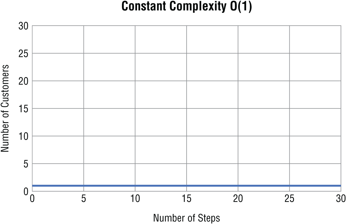
Figure 1.1 Constant complexity

Logarithmic Time

Logarithmic time is the second most efficient time complexity. An algorithm takes logarithmic time when its run time grows in proportion to the logarithm of the input size. You see this time complexity in algorithms such as a binary search that can discard many values at each iteration. If this is not clear, don't worry, because we will discuss this in depth later in the book. You express a logarithmic algorithm in big O notation as O(log n).

Figure 1.2 shows what it looks like when you plot a logarithmic algorithm.

The required number of steps grows more slowly in a logarithmic algorithm as the data set gets larger.

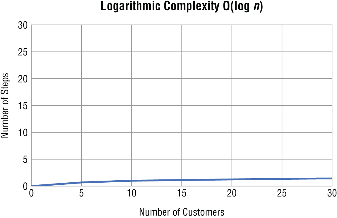
Figure 1.2 Logarithmic complexity

Linear Time

The next most efficient type of algorithm is one that runs in linear time. An algorithm that runs in linear time grows at the same rate as the size of the problem. You express a linear algorithm in big O notation as O(n).

Suppose you must modify your free book program so that instead of giving a free book to the first customer of the day, you iterate through your list of customers and give them a free book if their name starts with the letter B. This time, however, your list of customers isn't sorted alphabetically. Now you are forced to iterate through your list one by one to find the names that start with B.

When your customer list contains five items, your program takes five steps to complete. For a list of 10 customers, your program requires 10 steps; for 20 customers, 29 steps; and so on.

This is the equation for the time complexity of this program:

And in big O notation, you can ignore the constants and focus on the part that dominates the equation:

In a linear algorithm, as n gets bigger, the number of steps your algorithm takes increases by however much n increases (Figure 1.3).

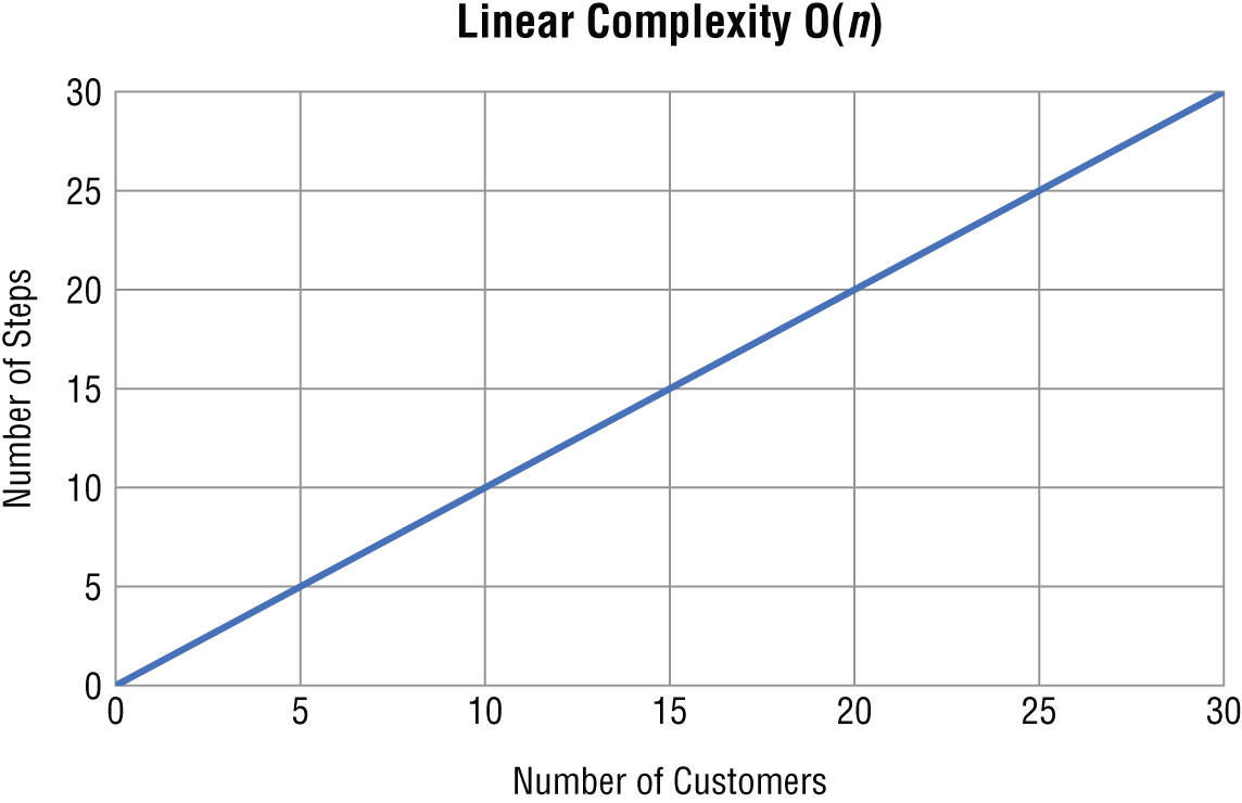
Figure 1.3 Linear complexity

Log-Linear Time

An algorithm that runs in log-linear time grows as a combination (multiplication) of logarithmic and linear time complexities. For example, a log-linear algorithm might evaluate an O(log n) operation n times. In big O notation, you express a log-linear algorithm as O(n log n). Log-linear algorithms often divide a data set into smaller parts and process each piece independently. For example, many of the more efficient sorting algorithms you will learn about later, such as merge sort, are log-linear.

Figure 1.4 shows what a log-linear algorithm looks like when you plot it on a graph.

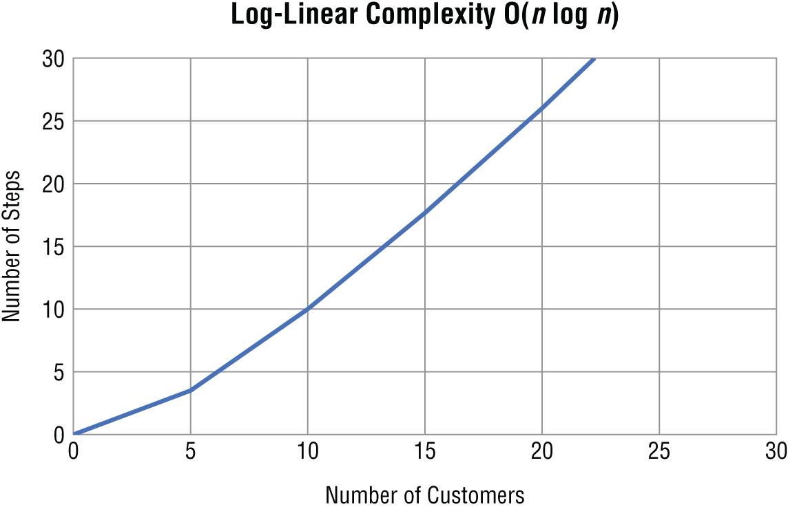
Figure 1.4 Log-linear complexity

As you can see, log-linear complexity is not as efficient as linear time. However, its complexity does not grow nearly as quickly as quadratic, which you will learn about next.

Quadratic Time

After log-linear, the next most efficient time complexity is quadratic time. An algorithm runs in quadratic time when its performance is directly proportional to the problem's size squared. In big O notation, you express a quadratic algorithm as O(n **2).

Here is an example of an algorithm with quadratic complexity:

This algorithm multiplies every number in a list of numbers by every other number, stores the result in a variable, and prints it.

In this case, n is the size of your numbers list. The equation for this algorithm's time complexity is as follows:

The (1 + 1) in the equation comes from the multiplication and print statement. You repeat the multiplication and print statement n * n times with your two nested for loops. You can simplify the equation to this:

which is the same as the following:

As you may have guessed, the n **2 part of the equation overshadows the rest, so in big O notation, the equation is as follows:

When you graph an algorithm with quadratic complexity, the number of steps increases sharply as the problem's size increases (Figure 1.5).

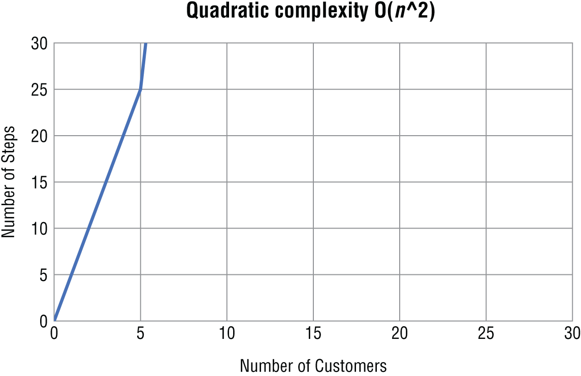
Figure 1.5 Quadratic complexity

As a general rule, if your algorithm contains two nested loops running from 1 to n (or from 0 to n − 1), its time complexity will be at least O(n **2). Many sorting algorithms such as insertion and bubble sort (which you will learn about later in the book) follow quadratic time.

Cubic Time

After quadratic comes cubic time complexity. An algorithm runs in cubic time when its performance is directly proportional to the problem's size cubed. In big O notation, you express a cubic algorithm as O(n **3). An algorithm with a cubic complexity is similar to quadratic, except n is raised to the third power instead of the second.

Here is an algorithm with cubic time complexity:

The equation for this algorithm is as follows:

Or as follows:

Like an algorithm with quadratic complexity, the most critical part of this equation is n **3, which grows so quickly it makes the rest of the equation, even if it included n **2, irrelevant. So, in big O notation, quadratic complexity is as follows:

While two nested loops are a sign of quadratic time complexity, having three nested loops running from 0 to n means that the algorithm will follow cubic time. You will most likely encounter cubic time complexity if your work involves data science or statistics.

Both quadratic and cubic time complexities are special cases of a larger family of polynomial time complexities. An algorithm that runs in polynomial time scales as O(n ** a), where a = 2 for quadratic time and a = 3 for cubic time. When designing your algorithms, you generally want to avoid polynomial scaling when possible because the algorithms can get very slow as n gets larger. Sometimes you can't escape polynomial scaling, but you can find comfort knowing that the polynomial complexity is still not the worst case, by far.

Exponential Time

The honor of the worst time complexity goes to exponential time complexity. An algorithm that runs in exponential time contains a constant raised to the size of the problem. In other words, an algorithm with exponential time complexity takes c raised to the n th power steps to complete. The big O notation for exponential complexity is O(c ** n), where c is a constant. The value of the constant doesn't matter. What matters is that n is in the exponent.

Fortunately, you won't encounter exponential complexity often. One example of exponential complexity involving trying to guess a numerical password consisting of n decimal digits by testing every possible combination is O(10** n).

Here is an example of password guessing with O(10** n) complexity:

The number of steps this algorithm takes to complete grows incredibly fast as n gets larger. When n is 1, this algorithm takes 10 steps. When n is 2, it takes 100 steps. When n is 3, it takes 1,000 steps. As you can see, at first, an exponential algorithm looks like it doesn't grow very quickly. However, eventually, its growth explodes. Guessing a password with 8 decimal digits takes 100 million steps, and guessing a password with 10 decimal digits takes more than 10 billion steps. Exponential scaling is the reason why it is so important to create long passwords. If someone tries to guess your password using a program like this, they can easily guess it if your password is four digits. However, if your password is 20 digits, it is impossible to crack because the program will take longer to run than a person's life span.

This solution to guessing a password is an example of a brute-force algorithm. A brute-force algorithm is a type of algorithm that tests every possible option. Brute-force algorithms are not usually efficient and should be your last resort.

Figure 1.6 compares the efficiency of the algorithms we have discussed.

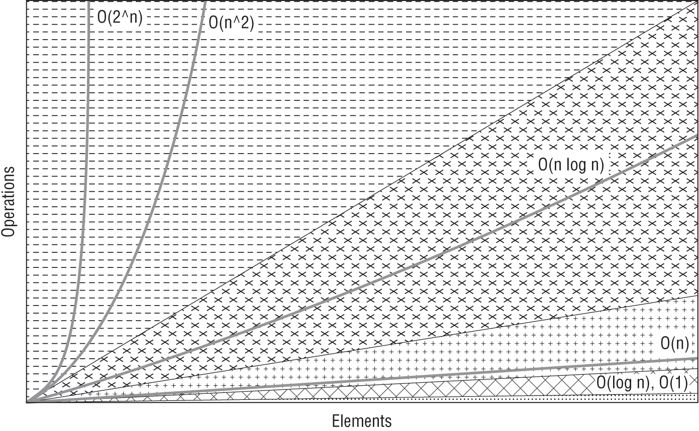
Figure 1.6 Big O complexity chart

Best-Case vs. Worst-Case Complexity

An algorithm's performance can change depending on different factors, such as the type of data you are working with. Because of this, when you evaluate an algorithm's performance, you need to consider its best-, worst-, and average-case complexities. An algorithm's best-case complexity is how it performs with ideal input, and an algorithm's worst-case complexity is how it performs in the worst possible scenario for it. An algorithm's average-case complexity is how it performs on average.

For example, if you have to search one by one through a list, you may get lucky and find what you are looking for after checking the first item in your list. That would be the best-case complexity. However, if the item you are looking for isn't in the list, you would have to search the entire list, which is the worst-case complexity.

If you have to search through a list one by one a hundred times, on average you will find what you are looking for in O(n /2) time, which is the same as O(n) time in big-O notation. When comparing algorithms, you often start by looking at the average-case complexity. If you want to do a deeper analysis, you can also compare their best-case and worst-case complexities.

Space Complexity

Computers have finite resources such as memory, so in addition to thinking about an algorithm's time complexity, you should consider its resource usage. Space complexity is the amount of memory space your algorithm needs and includes fixed space, data structure space, and temporary space. Fixed space is the amount of memory your program requires, and data structure space is the amount of memory your program needs to store the data set, for example, the size of a list you are searching. The amount of memory your algorithm uses to hold this data depends on the amount of input the problem requires. Temporary space is the amount of memory your algorithm needs for intermediary processing, for example, if your algorithm needs to temporarily copy a list to transfer data.

You can apply the time complexity concepts you learned earlier to space complexity. For example, you can calculate a factorial of n (a product of all positive integers less than or equal to n) using an algorithm that has a constant, O(1), space complexity:

The space complexity is constant because the amount of space your algorithm needs does not grow as n gets larger. If you decided to store all the factorials up to n in a list, your algorithm would have a linear space complexity, O(n):

Your algorithm's space complexity is O(n) because the amount of space it uses grows at the same pace as n.

Like with time complexity, the acceptable level of space complexity for an algorithm depends on the situation. In general, though, the less space an algorithm requires, the better.

Why Is This Important?

As a computer scientist, you need to understand the different orders of magnitude to optimize your algorithms. When you are trying to improve an algorithm, you should focus on changing its order of magnitude instead of improving it in other ways. For example, say you have an O(n **2) algorithm that uses two for loops. Instead of optimizing what happens inside your loops, it is much more important to determine whether you can rewrite your algorithm so that it doesn't have two nested for loops and thus has a smaller order of magnitude.

If you can solve the problem by writing an algorithm with two unnested for loops, your algorithm will be O(n), which will make a massive difference in its performance. That change will make a much bigger difference in your algorithm's performance than any efficiency gains you could get by tweaking your O(n **2) algorithm. However, it is also important to think about best- and worst-case scenarios for your algorithm. Maybe you have an O(n **2) algorithm, but in its best-case scenario, it is O(n), and your data happens to fit its best-case scenario. In that case, the algorithm may be a good choice.

The decisions you make about algorithms can have enormous consequences in the real world. For example, say you are a web developer responsible for writing an algorithm that responds to a customer's web request. Whether you decide to write a constant or quadratic algorithm could make the difference between your website loading in less than one second, making your customer happy, and taking more than a minute, which may cause you to lose customers before the request loads.

Vocabulary

• algorithm: A sequence of steps that solves a problem.
• run time: The amount of time it takes your computer to execute an algorithm written in a programming language like Python.
• size of the problem: The variable n in an equation that describes the number of steps in an algorithm.
• big O notation: A mathematical notation that describes how an algorithm's time or space requirements increase as the size of n increases.
• order of magnitude: A class in a classification system where each class is many times greater or smaller than the one before.
• time complexity: The maximum number of steps an algorithm takes to complete as n gets larger.
• constant time: An algorithm runs in constant time when it requires the same number of steps regardless of the problem's size.
• logarithmic time: An algorithm runs in logarithmic time when its run time grows in proportion to the logarithm of the input size.
• linear time: An algorithm runs in linear time when it grows at the same rate as the problem's size.
• log-linear time: An algorithm runs in log-linear time when it grows as a combination (multiplication) of logarithmic and linear time complexities.
• quadratic time: An algorithm runs in quadratic time when its performance is directly proportional to the square of the size of the problem.
• cubic time: An algorithm runs in cubic time when its performance is directly proportional to the cube of the size of the problem.
• polynomial time: An algorithm runs in polynomial time when it scales as O(n ** a), where a = 2 for quadratic time and a = 3 for cubic time.
• exponential time: An algorithm runs in exponential time when it contains a constant raised to the problem's size.
• brute-force algorithm: A type of algorithm that tests every possible option.
• best-case complexity: How an algorithm performs with ideal input.
• worst-case complexity: How an algorithm performs in the worst possible scenario for it.
• average-case complexity: How an algorithm performs on average.
• space complexity: The amount of memory space an algorithm needs.
• fixed space: The amount of memory a program requires.
• data structure space: The amount of memory a program requires to store the data set.
• temporary space: The amount of memory an algorithm needs for intermediary processing, for example, if your algorithm needs to temporarily copy a list to transfer data.

Challenge

1. Find a program you've written in the past. Go through it and write down the time complexities for the different algorithms in it.