SELECT Statement, we broke the SELECT statement down into its various clauses, but looked at each clause only briefly. In this chapter, we’ll begin our more detailed look at the SELECT statement, starting with the FROM clause.
The FROM clause can be simple, and it can also be quite complex. In all cases, though, the important point about the FROM clause is that it produces a tabular structure. This tabular structure is referred to as the result set of the FROM clause. You may also see it referred to as an intermediate result set, an intermediate tabular result set, or an intermediate table. But, no matter whether the SELECT query retrieves data from one table, from many tables, or from other, similar tabular structures, the result is always the same – the FROM clause produces a tabular structure.
In this chapter we’ll review the common types of FROM clause that we might encounter in web development.
Why Start with the FROM Clause?
To begin writing aSELECT statement, my strategy is to skip over the SELECT clause for the time being, and write the FROM clause first. Eventually, we’ll need to input some expressions into the SELECT clause and we might also need to use WHERE, GROUP BY, and the other clauses too. But there are good reasons why we should always start with the FROM clause:
- If we get the
FROMclause wrong, the SQL statement will always return the wrong results. It’s theFROMclause that produces the tabular structure, the starting set of data on which all other operations in aSELECTstatement are performed. - The
FROMclause is the first clause that the database system looks at when it parses the SQL statement.
Parsing an SQL Statement
Whenever we send an SQL statement to the database system to be executed, the first action that the system performs is called parsing. This is how the database system examines the SQL statement to see if it has any syntax errors. First it divides the statement into its component clauses; then it examines each clause according to the syntax rules for that clause. Contrary to what we might expect, the database system parses theFROM clause first, rather than the SELECT clause.
For example, suppose we were to attempt to run the following SQL statement, in which we have misspelled teams as teans:
SELECT
  id, name
FROM
  teans
WHERE
conference = 'F'FROM clause refers to a non-existing table, so there is an immediate syntax error. If the database system were to parse the SELECT clause first, it would need to examine the table definitions of all the tables in the database, looking for one that might contain two columns called name and id. In fact, it’s quite common for a database to have several tables with two columns called name and id. Confusion could ensue and the database would require more information from us to know which table to retrieve name and id from. Hence why the database system parses the FROM clause first, and this is the first clause we think about as well.
FROM One Table
We’ve already seen theFROM clause with a single table. In Chapter 1, An Introduction to SQL, we saw the FROM clause specify the teams table:
SELECT
  id, name
FROM
teamsSELECT
title, category
FROM
entriesFROM More than One Table Using JOINs
A join relates, associates, or combines two tables together. A join starts with two tables, then combines – or joins – them together in one of several different ways, producing a single tabular structure (as the result of the join). Actually, the verb ‘to join’ is very descriptive of what happens, as we’ll see in a moment. The way that the tables are joined – the type of join – is specified in theFROM clause using special keywords as well as the keyword JOIN. There are several different types of join, which I’ll describe briefly, so that you can see how they differ. Then we’ll look at specific join examples, using our sample applications.
Types of Join
A join combines the rows of two tables, based on a rule called a join condition; this compares values from the rows of both tables to determine which rows should be joined. There are three basic types of join:- inner join, created with the
INNER JOINkeywords - outer join, which comes in three varieties:
LEFT OUTER JOINRIGHT OUTER JOINFULL OUTER JOIN
- cross join, created with the
CROSS JOINkeywords
 On Tables A and B
These tables are actually oversimplified, because they blur the distinction between table and column names. The join condition actually specifies the columns that must match. Further, it’s unusual for tables to have just one column.
Don’t worry about what
On Tables A and B
These tables are actually oversimplified, because they blur the distinction between table and column names. The join condition actually specifies the columns that must match. Further, it’s unusual for tables to have just one column.
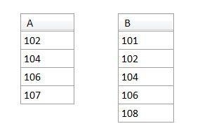
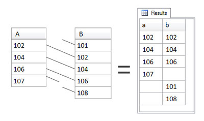
Don’t worry about what A and B might actually represent. They could be anything. The idea in the following illustrations is for you to focus your attention on the values in the rows being joined. Table A has one column called a and rows with values 102, 104, 106, and 107. Table B has one column called b and rows with values 101, 102, 104, 106, and 108.
The Inner Join
For an inner join, only rows satisfying the condition in the ON clause are returned. Inner joins are the most common type of join. In most cases, such as the example below, the ON clause specifies that two columns must have matching values. In this case, if the value (of column a) in a row from one table (A) is equal to the value (of column b) in a row from the other table (B), the join condition is satisfied, and those rows are joined:SELECT
a, b
FROM
A INNER JOIN B
ON a=b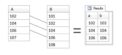 As you can see, a row from
 A is joined to a row from B when their values are equal. Thus values 102, 104, and 106 are returned in the result set. Value 107 in A has no match in B, and therefore is not included in the result set. Similarly, the values 101 and 108 in B have no match in A, so they’re not included in the result set either. If it’s easier to do so, you can think of it as though the matching rows are actually concatenated into a single longer row on which the rest of the SELECT statement then operates.
Outer Joins
Next, we’ll look at outer joins. Outer joins differ from inner joins in that unmatched rows can also be returned. As a result, most people say that an outer join includes rows that don’t match the join condition. This is correct, but might be a bit misleading, because outer joins do include all rows that match. Typical outer joins have many rows that match, and only a few that don’t. There are three different types of outer join: left, right, and full. We’ll start with the left outer join.The Left Outer Join
For a left outer join, all rows from the left table are returned, regardless of whether they have a matching row in the right table. Which one’s the left table, and which one’s the right table? These are simply the tables mentioned to the left and to the right of theOUTER JOIN keywords. For example, in the following statement, A is the left table and B is the right table and a left outer join is specified in the FROM clause:
SELECT
a, b
FROM
A LEFT OUTER JOIN B
ON a=b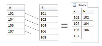 Notice that all values from
 A are returned. This is because A is the left table. In the case of 107, which did not have a match in B, we see that it is indeed included in the results, but there is no value in that particular result row from B. For the time being, it’s okay just to think of the value from B as missing – which, of course, for 107 it is.
The Right Outer Join
For a right outer join, all rows from the right table are returned, regardless of whether they have a match in the left table. In other words, a right outer join works exactly like a left outer join, except that all the rows of the right table are returned instead:SELECT
a, b
FROM
A RIGHT OUTER JOIN B
ON a=bA is still the left table and B is still the right table, because that’s where they are mentioned in relation to the OUTER JOIN keywords. Consequently, the result of the join contains all the rows from table B, together with matching rows of table A, if any, as shown in Figure 3.4, “A RIGHT OUTER JOIN B”.
 The right outer join is the reverse of the left outer join. With the same tables in the same positions –
 A as the left table and B as the right table – the results of the right outer join are very different from those of a left outer join. This time, all values from B are returned. In the case of 101 and 108, which did not have a match in A, they are indeed included in the results, but there is no value in their particular result rows from A. Again, those values from A are missing, but the row is still returned.
The Full Outer Join
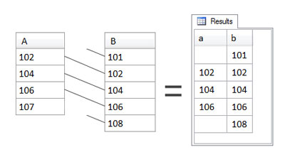
For a full outer join, all rows from both tables are returned, regardless of whether they have a match in the other table. In other words, a full outer join works just like left and right outer joins, except this time all the rows of both tables are returned. Consider this example:SELECT
a, b
FROM
A FULL OUTER JOIN B
ON a=bA is the left table and B is the right table, although this time it doesn’t really matter. Full outer joins return all rows from both tables, together with matching rows of the other table, if any, as shown below.
 The full outer join is a combination of left and right outer joins. (More technically, if you remember your set theory from mathematics at school, it’s the union of the results from the left and right outer joins.) Matching rows are – of course – included, but rows that have no match from either table, are also included.
The Difference between Inner and Outer Joins
The results of an outer join will always equal the results of the corresponding inner join between the two tables plus some unmatched rows from either the left table, the right table, or both – depending on whether it is a left, right, or full outer join, respectively. Thus the difference between a left outer join and a right outer join is simply the difference between whether the left table’s rows are all returned, with or without matching rows from the right table, or whether the right table’s rows are all returned, with or without matching rows from the left table. A full outer join, meanwhile, will always include the results from both left and right outer joins.The Cross Join
For a cross join, every row from both tables is returned, joined to every row of the other table, regardless of whether they match. The distinctive feature of a cross join is that it has no ON clause – as you can see in the following query:SELECT
a, b
FROM
A CROSS JOIN B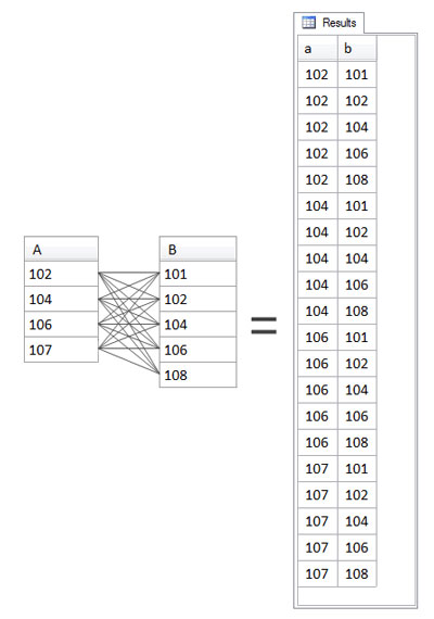 Cross joins can be very useful but are exceedingly rare. Their purpose is to produce a tabular structure containing rows which represent all possible combinations of two sets of values (in our example, columns from two tables) as shown in Figure 3.6, “A CROSS JOIN B”; this can be useful in generating test data or looking for missing values.
Old-Style Joins
There’s another type of join, which has a comma-separated list of tables in theFROM clause, with the necessary join conditions in the WHERE clause; this type of join is sometimes called the “old-style” join, or “comma list” join, or “WHERE clause” join. For example, for the A and B tables, it would look like this:
SELECT
a, b
FROM
A, B
WHERE
a=bINNER JOIN:
SELECT
  a, b
FROM
  A INNER JOIN B
ON a=bJOIN syntax.
To recap our quick survey of joins, there are three basic types of join and a total of five different variations:
- inner join
- left outer join, right outer join, and full outer join
- cross join
Real World Joins
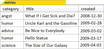
Chapter 2, An Overview of theSELECT Statement introduced the Content Management System entries table, which we’ll continue to use in the following queries to demonstrate how to write joins. Figure 3.7, “The entries table” shows some – but not all – of its contents. The content column, for example, is missing.
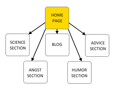
 Within our CMS web site, the aim is to give each category its own area on the site, linked from the site’s main menu and front page. The science area will contain all the entries in the science category, the humor area will contain all the entries in the humor category, and so on, as shown in Figure 3.8, “A suggested CMS site structure”. To this end, each entry is given a category, stored in the category column of each row.
 The main category pages themselves would need more than just the one word category name that we see in the entries table. Site visitors will want to understand what each section is about, so we’ll need a more descriptive name for each category. But where to store this in the site? We could hardcode the longer name directly into each main section page of the web site. A better solution, however, would be to save the names in the database. Another table will do the job nicely, and so we create the categories table for this purpose; we’ll give it two columns – category and name – as shown in Figure 3.9, “The categories table”.
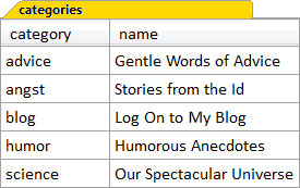 The category column is the key to each row in the categories table. It’s called a key because the values in this column are unique, and are used to identify each row. This is the column that we’ll use to join to the entries table. We’ll learn more about designing tables with keys in Chapter 10, Relational Integrity. Right now, let’s explore the different ways to join the categories and entries tables.
Creating the Categories Table
The script to create the categories table can be found in Appendix C, Sample Scripts and in the download for the book in a file called CMS_05_Categories_INNER_JOIN_Entries.sql.Inner Join: Categories and Entries
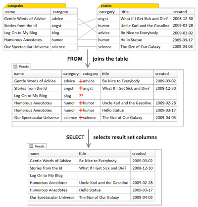
The first join type we’ll look at is an inner join:SELECT
categories.name, entries.title, entries.created
FROM
  categories
    INNER JOIN entries
ON entries.category = categories.category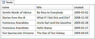 Let’s walk through the query clause by clause and examine what it’s doing, while comparing the query to the results it produces. The first part of the query to look at, of course, is the
 FROM clause:
FROM
categories
INNER JOIN entries
ON entries.category = categories.categoryINNER JOIN. The ON clause specifies the join condition, which dictates how the rows of the two tables must match in order to participate in the join. It uses dot notation (tablename.rowname) to specify that rows of the categories table will match rows of the entries table only when the values in their category columns are equal. We’ll look in more detail at dot notation later in this chapter.
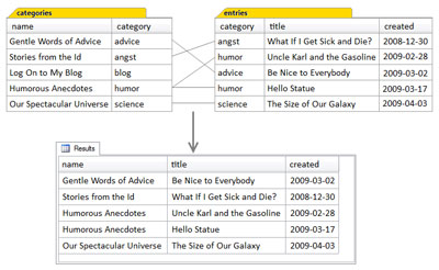
The figure below shows in detail how the result set of the query is produced by the inner join of the categories table to the entries table. Because it’s an inner join, each of the rows of the categories table is joined only to the rows of the entries table that have matching values in their respective category columns.
 Some of the Entries Table is Hidden
The entries table actually has several additional columns that are not shown: id, updated, and content. These columns are also available, but were omitted to keep the diagram simple. In fact, the diagram would’ve been quite messy if the content column had been included, as it contains multiple lines of text. Since these columns were not mentioned in the query at all, including them in the diagram might have made it confusing. Some readers would surely ask, “Hey, where did these come from?”
Some of the Entries Table is Hidden
The entries table actually has several additional columns that are not shown: id, updated, and content. These columns are also available, but were omitted to keep the diagram simple. In fact, the diagram would’ve been quite messy if the content column had been included, as it contains multiple lines of text. Since these columns were not mentioned in the query at all, including them in the diagram might have made it confusing. Some readers would surely ask, “Hey, where did these come from?”
- Regarding the matching of rows of the categories and entries tables, notice that: The categories row for humor matched two entries rows, and both instances of matched rows are in the results, with the name of the humor category appearing twice.
- The categories row for blog matched no entries rows. Consequently, as this is an inner join, this category does not appear in the results.
- The other categories rows matched one entries row each, and these matched rows are in the result.
FROM clause and seen how the INNER JOIN and its ON condition have specified how the tables are to be joined, we can look at the SELECT clause:
SELECT
  categories.name
, entries.title
, entries.createdSELECT clause simply specifies which columns from the result of the inner join are to be included in the result set.
Leading Commas
Notice that theSELECT clause has now been written with one line per column, using a convention called leading commas; this places the commas used to separate the second and subsequent items in a list at the front of their line. This may look unusual at first, but the syntax is perfectly okay; remember, new lines and white space are ignored by SQL just as they are by HTML. Experienced developers may be more used to having trailing commas at the end of the lines, like this:
SELECT
  categories.name,
  entries.title,
entries.createdSELECT
first_name,
last_name,
title
position,
staff_id,
group,
region,
FROM
staffSELECT
first_name
, last_name
, title
position
, pay_scale
, group
, region
,
FROM
staffSELECT clause, and it’s easier to select (highlight) the single line with the keyboard’s Shift and Arrow keys. Similarly, removing the last column requires also removing the trailing comma from the previous line, which is easy to forget. A dangling comma in front of the FROM keyword is a common error that’s difficult to make using leading commas.
All Columns Are Available after a Join
In any join, all columns of the tables being joined are available to theSELECT query, even if they’re not used by the query. Let’s look at our inner join again:
SELECT
  categories.name
, entries.title
, entries.created
FROM
  categories
    INNER JOIN entries
ON entries.category = categories.categorySELECT clause. This is true here too; the entries table has other columns not mentioned in the query. We haven’t included them in Figure 3.11, “The inner join in detail” just to keep the figure simple. Although the figure is correct, it could be construed as slightly misleading, because it shows only the result set of the query, rather than the tabular structure produced by the inner join.
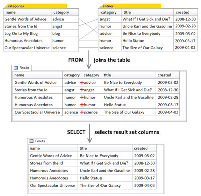
The figure below expands on the actual processing of the query and shows the tabular structure that’s produced by the FROM clause and the inner join; it includes the two category columns – one from each table. This tabular structure, the intermediate table, is produced by the database system as it performs the join, and held temporarily for the SELECT clause.
When a Join is Executed in a Query
Two important points come out of the analysis of our first example join query:- A join produces an intermediate tabular result set;
- The SELECT clause occurs after the
FROMclause and operates on the intermediate result set.
FROM clause is the first clause that the database system parses when we submit a query. If there are no syntax errors, the database system goes ahead and executes the query. Well, it turns out that the FROM clause is the first clause that the database system executes, too.
You could consider the execution of a join query as working in the following manner. First, the database system produces an intermediate tabular result set based on the join specified in the FROM clause. This contains all the columns from both tables. Then the database system uses the SELECT clause to select only the specified columns from this intermediate result set, and extracts them into the final tabular structure that is returned as the result of the query.
Qualifying Column Names
Finally, let’s take one more look at our inner join query:SELECT
categories.name
, entries.title
, entries.created
FROM
categories
INNER JOIN entries
ON entries.category = categories.categorySELECT
name
, title
, created
FROM
categories
INNER JOIN entries
ON entries.category = categories.categorySELECT clause, you can’t always tell which table each column comes from. This can be especially frustrating if you’re only remotely familiar with the tables involved in the query, such as when you’re troubleshooting a query written by another person (or even by yourself, a few months ago).
Always Qualify Every Column in a Join Query
Even though some or even all columns may not need to be qualified within a join query, qualifying every column in a multi-table query is part of good SQL coding style, because it makes the query easier for us to understand. In a way, qualifying column names makes the query self-documenting: it makes it obvious what the query is doing so that it’s easier to explain in documentation.Table Aliases
Another way to qualify column names is by using table aliases. A table alias is an alternate name assigned to a table in the query. In practice, a table alias is often shorter than the table name. For example, here’s the same inner join using table aliases:SELECT
cat.name
, ent.title
, ent.created
FROM
categories AS cat
INNER JOIN entries AS ent
ON ent.category = cat.categoryLeft Outer Join: Categories and Entries
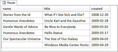
Continuing our look at join queries, the left outer join query we’ll examine is exactly the same as the inner join query we just covered, except that it usesLEFT OUTER JOIN as the join keywords:
SELECT
categories.name
, entries.title
, entries.created
FROM
categories
LEFT OUTER JOIN entries
ON entries.category = categories.category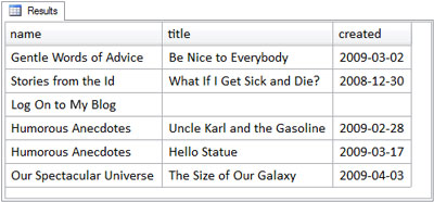 The only difference between this left outer join query and the preceding inner join query is the inclusion of one additional row – for the category with the name Log On to My Blog – in the result set. The additional row is included because the query uses an outer join. Specifically, it’s a left outer join, and therefore all of the rows of the left table, the categories table, must be included in the results. The left table, you may recall, is simply the table that is mentioned to the left of the
 LEFT OUTER JOIN keywords. The figure below shows the process of the join and selection in more detail.
 To make it more obvious which table is the left one and which table is the right one, we could write the join without line breaks and spacing so categories is more obviously the left table in this join:
FROM categories LEFT OUTER JOIN entriesAn Application for Left Outer Joins: a Sitemap
Looking at the results of ourLEFT OUTER JOIN query, it’s easy enough to see how they could form the basis of a sitemap for the CMS. For example, the HTML for the sitemap that can be produced by these query results might be:
<h2>Gentle Words of Advice</h2>
<ul>
  <li>Be Nice to Everybody (2009-03-02)</li>
</ul>

<h2>Stories from the Id</h2>
<ul>
  <li>What If I Get Sick and Die? (2008-12-30)</li>
</ul>

<h2>Log On to My Blog</h2>

<h2>Humorous Anecdotes</h2>
<ul>
  <li>Hello Statue (2009-03-17)</li>
  <li>Uncle Karl and the Gasoline (2009-02-28)</li>
</ul>

<h2>Our Spectacular Universe</h2>
<ul>
  <li>The Size of Our Galaxy (2009-04-03)</li>
</ul> NULLs in the entries columns of that result row.
Outer Joins Produce NULLs
Our left outer join includes rows from the left table that have no match in the right table, as shown in Figure 3.13, “The results of the left outer join query”. So what exactly are the values in the title and created columns of the blog category result row? Remember, these columns come from the entries table. The answer is: they areNULL.
NULL is a special value in SQL, which stands for the absence of a value. In a left outer join, columns that come from the right table for unmatched rows from the left table are NULL in the result set. This literally means that there is no value there, which makes sense because there is no matching row from the right table for that particular row of the left table.
Working with NULLs is part of daily life when it comes to working with databases. We first came across NULL (albeit briefly) in Chapter 1, An Introduction to SQL, where it was used in a sample CREATE TABLE statement and we’ll see NULL again throughout the book.
Right Outer Join: Entries and Categories
The following right outer join query produces exactly the same results as the left join query we just covered:SELECT
categories.name
, entries.title
, entries.created
FROM
entries
RIGHT OUTER JOIN categories
ON entries.category = categories.categoryFROM entries RIGHT OUTER JOIN categoriesFROM categories LEFT OUTER JOIN entriesRight Outer Join: Categories and Entries
What if I hadn’t switched the order of the tables in the preceding right outer join? Suppose the query had been:SELECT
categories.name
, entries.title
, entries.created
FROM
categories
RIGHT OUTER JOIN entries
ON entries.category = categories.category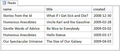 How can this be? Is this more deviousness? No, not this time; the reason is because it’s the actual contents of the tables. Remember, a right outer join returns all rows of the right table, with or without matching rows from the left table. The entries table is the right table, but in this particular instance, every entry has a matching category. All the entries are returned, and there are no unmatched rows.
So it wasn’t really devious to show that the right outer join produces the same results as the inner join, because it emphasized the rule for outer joins that all rows from the outer table are returned, with or without matching rows, if any. In this case, there weren’t any.
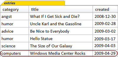
To really see the right outer join in action, we’d need an entry that lacks a matching category. Let’s add an entry to the entries table, for a new category called computers, as shown in the figure below.
How can this be? Is this more deviousness? No, not this time; the reason is because it’s the actual contents of the tables. Remember, a right outer join returns all rows of the right table, with or without matching rows from the left table. The entries table is the right table, but in this particular instance, every entry has a matching category. All the entries are returned, and there are no unmatched rows.
So it wasn’t really devious to show that the right outer join produces the same results as the inner join, because it emphasized the rule for outer joins that all rows from the outer table are returned, with or without matching rows, if any. In this case, there weren’t any.
To really see the right outer join in action, we’d need an entry that lacks a matching category. Let’s add an entry to the entries table, for a new category called computers, as shown in the figure below.
Trying Out Your SQL
TheINSERT statement that adds this extra row to the entries table can be found in the section called “Content Management System”.
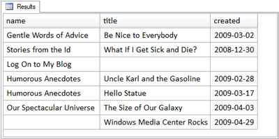
Figure 3.17, “The results of the right outer join query – take two” shows that when we re-run the right outer join query with the new category, the results are as expected.
 This time, we see the unmatched entry in the query results, because there’s no row in the categories table for the computers category.
Full Outer Join: Categories and Entries
Our next example join query is the full outer join. The full outer join query syntax, as I’m sure you can predict, is remarkably similar to the other join types we’ve seen so far:SELECT
categories.name
, entries.title
, entries.created
FROM
categories
FULL OUTER JOIN entries
ON entries.category = categories.categoryFULL OUTER JOIN, but an unfortunate error happens in at least one common database system. In MySQL, which doesn’t support FULL OUTER JOIN despite it being standard SQL, the result is a syntax error: SQL Error: You have an error in your SQL syntax; check the manual that corresponds to your MySQL server version for the right syntax to use near ‘OUTER JOIN entries ON …’
The figure below shows the result in other database systems that do support FULL OUTER JOIN.
 Notice that the result set includes unmatched rows from both the left and the right tables. This is the distinguishing feature of full outer joins that we saw earlier; both tables are outer tables, so unmatched rows from both are included. It’s for this reason that full outer joins are rare in web development as there are few situations that call for them. In contrast, inner joins and left outer joins are quite common.
UNION Queries
If your database system does not support theFULL OUTER JOIN syntax, the same results can be obtained by a slightly more complex query, called a union. Union queries are not joins per se. However, most people think of the results produced by a union query as consisting of two results sets concatenated or appended together. UNION queries perform a join only in a very loose sense of the word.
Let’s have a look at a union query:
SELECT
categories.name
, entries.title
, entries.created
FROM
categories
LEFT OUTER JOIN entries
ON entries.category = categories.category
UNION
SELECT
  categories.name
, entries.title
, entries.created
FROM
  categories
    RIGHT OUTER JOIN entries
ON entries.category = categories.categoryUNION keyword. A union query consists of a number of SELECT statements combined with the UNION operator. They’re called subselects in this context because they’re subordinate to the whole UNION query; they’re only part of the query, rather than being a query executed on its own. Sometimes they’re also called subqueries, although this term is generally used for a more specific situation, which we shall meet shortly.
When executed, a UNION operation simply combines the result sets produced by each of its subselect queries into a single result set. Figure 3.19, “How a union query works” shows how this works for the example above:
I mentioned earlier that a join operation can best be imagined as actually concatenating a row from one table onto the end of a row from the other table – a horizontal concatenation, if you will. The union operation is therefore like a vertical concatenation – a second result set is appended onto the end of the first result set.
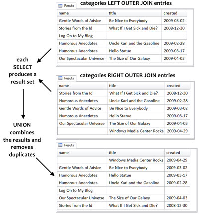 The interesting feature is that duplicates are removed. You can see the duplicates easily enough – they are entire rows in which every column value is identical. The reason that duplicates are produced in this example is due to both of the sub-selects – the left outer join and the right outer join – returning rows from the same two tables which match the the same join conditions. Thus, matched rows are returned by both subselects, creating duplicate rows in the intermediate results. Only the unmatched rows are not duplicated.
You might wonder why
The interesting feature is that duplicates are removed. You can see the duplicates easily enough – they are entire rows in which every column value is identical. The reason that duplicates are produced in this example is due to both of the sub-selects – the left outer join and the right outer join – returning rows from the same two tables which match the the same join conditions. Thus, matched rows are returned by both subselects, creating duplicate rows in the intermediate results. Only the unmatched rows are not duplicated.
You might wonder why UNION removes duplicates; the answer is simply that it’s designed that way. It’s how the UNION operator is supposed to work.
UNION and UNION ALL
Sometimes it’s important to retain all rows produced by a union operation, and not have the duplicate rows removed. This can be accomplished by using the keywordsUNION ALL instead of UNION.
UNIONremoves duplicate rows. Only one row from each set of duplicate rows is included in the result set.UNION ALLretains all rows produced by the subselects of the union, maintaining duplicate rows.
UNION ALL is significantly faster because the need to search for duplicate rows – in order to remove them – is redundant.
The fact that our union query removed the duplicate rows means that the above union query produces the same results as the full outer join. Of course, this example was contrived to do just that.
There is more to be said about union queries, but for now, let’s finish this section with one point: union queries, like join queries, produce a tabular structure as their result set.
Views
A view is another type of database object that we can create, like a table. Views are insubstantial, though, because they don’t actually store data (unlike tables). Views areSELECT statements (often complex ones) that have been given a name for ease of reference and reuse, and can be used for many purposes:
- They can customize a
SELECTstatement, by providing column aliases. - They can be an alias to the result set produced by the
SELECTstatement in their definition. If theSELECTstatement in the view contains joins between a number of tables, they are effectively pre-joined by the database in advance of a query against the view. All this second query then sees is a single table to query against. This is probably the most important benefit of using views. - They can enforce security on the database. Users of a database might be restricted from looking at the underlying tables altogether; instead, they might only be granted access to views. The classic example is the employees table, which contains columns like name, department, and salary. Because of the confidential nature of salary, very few people are granted permission to access such a table directly; rather, a special view is made available that excludes the confidential columns.
SELECT
  categories.name
, entries.title
, entries.created
FROM
  categories
    LEFT OUTER JOIN entries
      ON entries.category = categories.category
UNION
SELECT
  categories.name
, entries.title
, entries.created
FROM
  categories
    RIGHT OUTER JOIN entries
ON entries.category = categories.categorySELECT statement. The use of the view name here works by executing the view’s underlying SELECT statement, storing its results in an intermediate table, and using that table as the result of the FROM clause. The results of the above query, shown below.
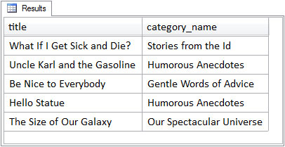 This result set is similar to the result set produced by the inner join query which defines the view. Notice that only two columns have been returned, because the
 SELECT statement which uses the view in its FROM clause (as opposed to the SELECT statement which defines the view) only asked for two. Also, notice that a column alias called category_name was assigned to the categories table’s name column in the view definition; this is the column name that must be used in any SELECT statement which uses the view, and it’s the column name used in the result set.
One particular implication of the view definition is that only the columns defined in the view’s SELECT statement are available to any query that uses the view. Even though the entries table has a content column, this column is unknown to the view and will generate a syntax error if referenced in a query using the view.
Views in Web Development
How do views relate to our day-to-day tasks as web developers?- When working on a large project in a team environment, you may be granted access to views only, not the underlying tables. For example, a Database Administrator (DBA) may have built the database, and you’re just using it. You might not even be aware that you’re using views. This is because, syntactically, both tables and views are used in the
FROMclause in exactly the same way. - When you build your own database, you may wish to create views for the sake of convenience. For example, if you often need to display a list of entries and their category on different pages within the site, it’s a lot easier to write
FROMentries_with_category than the underlying join.
Subqueries and Derived Tables
We started this chapter by examining theFROM clause, working our way up from simple tables through the various types of joins. We briefly saw a UNION query and its subselects, and we’ve also seen how views make complex join expressions easier to use. To finish this chapter, we’ll take a quick look at derived tables. Here’s an example:
SELECT
  title
, category_name
FROM
  ( SELECT
      entries.title
    , entries.created
    , categories.name AS category_name
    FROM
      entries
        INNER JOIN categories
          ON categories.category = entries.category
) AS entries_with_categorySELECT query in parentheses (the parentheses are required in the syntax, to delimit the enclosed query). A derived table is a common type of subquery, which is a query that’s subordinate to – or nested within – another query (much like the subselects in the union query).
It looks familiar, too, doesn’t it? This subquery is the same query used in the entries_with_categories view defined in the previous section. Indeed, just as every view needs a name, every derived table must be also given a name, also using the AS keyword (on the last line) to assign the name entries_with_category as a table alias for the derived table. With these similarities in mind, derived tables are often also called inline views. That is, they define a tabular structure – the result set produced by the subquery – directly inline in (or within) the SQL statement, and the tabular structure produced by the subquery, in turn, is used as the source of the data for the FROM clause of outer or main query.
In short, anything which produces a tabular structure can be specified as a source of data in the FROM clause. Even a UNION query, which we discussed briefly, can also be used in the FROM clause, if it’s specified as a derived table; the entire UNION query would go into the parentheses that delimit the derived table.
Derived tables are incredibly useful in SQL. We’ll see several of them throughout the book.
Wrapping Up: the FROM Clause
In this chapter, we examined theFROM clause, and how it specifies the source of the data for the SELECT statement. There are many different types of tabular structures that can be specified in the FROM clause:
- single tables
- joined tables
- views
- subqueries or derived tables
FROM clause specify one or more tabular structures from which to extract data, but the result of the execution of the FROM clause is also another tabular structure, referred to as the intermediate result set or intermediate table. In general, this intermediate table is produced first, before the SELECT clause is processed by the database system.
In the Chapter 4, The WHERE Clause, we’ll see how the WHERE clause can be used to filter the tabular structure produced by the FROM clause.
Hope you enjoyed that sample chapter. If you’d like to read some more from Simply SQL you can download the sample PDF, which contains 3 chapters, or go and buy the book!
Frequently Asked Questions about SQL FROM Clause
What is the purpose of the FROM clause in SQL?
The FROM clause in SQL is used to specify the table from which data is to be retrieved. It is an essential part of the SELECT statement, which is used to fetch data from a database. The FROM clause is followed by the name of the table from which you want to fetch the data. If you want to fetch data from multiple tables, you can list them separated by commas.
Can I use multiple tables in the FROM clause?
Yes, you can use multiple tables in the FROM clause. This is often done when you need to join tables to fetch related data. The tables are listed in the FROM clause, separated by commas. The data from these tables can then be combined in various ways using different types of joins, such as INNER JOIN, LEFT JOIN, RIGHT JOIN, and FULL JOIN.
What is the difference between a CROSS JOIN and other types of joins?
A CROSS JOIN in SQL is a type of join that produces a Cartesian product of the tables involved. It returns all possible combinations of rows from the two tables. Unlike other types of joins, a CROSS JOIN does not require a condition to match rows from the joined tables. On the other hand, INNER JOIN, LEFT JOIN, RIGHT JOIN, and FULL JOIN return rows based on matching conditions.
How does the FROM clause work in Oracle DB?
In Oracle DB, the FROM clause works similarly to other SQL databases. It is used to specify the table or tables from which data is to be retrieved. You can list multiple tables in the FROM clause to join them and fetch related data. Oracle DB also supports various types of joins, including INNER JOIN, LEFT JOIN, RIGHT JOIN, FULL JOIN, and CROSS JOIN.
Can I use subqueries in the FROM clause?
Yes, you can use subqueries in the FROM clause. A subquery in the FROM clause defines a temporary table that can be used within the scope of the outer SELECT statement. This can be useful when you need to perform complex queries that involve operations on multiple sets of data.
What is the order of execution of SQL clauses?
The order of execution of SQL clauses is as follows: FROM, WHERE, GROUP BY, HAVING, SELECT, ORDER BY. This means that the FROM clause is executed first. It specifies the table or tables from which data is to be retrieved. The WHERE clause then filters the data based on certain conditions. The GROUP BY clause groups the data, and the HAVING clause filters the grouped data. The SELECT clause specifies the columns to be returned, and the ORDER BY clause sorts the result.
How can I use aliases in the FROM clause?
You can use aliases in the FROM clause to give a table or a subquery a temporary name. This can make your SQL code more readable and easier to maintain. To create an alias, you simply follow the table or subquery with the alias name. You can then use this alias in other parts of your SQL statement.
What is the difference between the FROM clause and the JOIN clause?
The FROM clause and the JOIN clause are both used to combine data from multiple tables. However, they do it in different ways. The FROM clause lists the tables to be joined, separated by commas. The JOIN clause, on the other hand, specifies the type of join and the condition for matching rows from the joined tables.
Can I use the FROM clause without the SELECT statement?
No, you cannot use the FROM clause without the SELECT statement. The FROM clause is an integral part of the SELECT statement. It specifies the table or tables from which data is to be retrieved. Without the SELECT statement, the FROM clause has no context and would result in an error.
How can I optimize the performance of queries using the FROM clause?
There are several ways to optimize the performance of queries using the FROM clause. One way is to limit the number of tables listed in the FROM clause. Joining too many tables can lead to performance issues. Another way is to use indexes on the columns that are used in the join conditions. This can significantly speed up the query execution. Also, consider using subqueries in the FROM clause for complex queries, as they can sometimes be more efficient than joins.
 Rudy Limeback
Rudy Limeback is an SQL Consultant living in Toronto, Canada. His SQL experience spans 20+ years, and includes working with DB2, SQL Server, Access, Oracle, and MySQL. He is an avid participant in discussion forums, primarily at SitePoint. His two web sites are http://r937.com/ and http://rudy.ca/.


